Lumos Video Store
This page provides a list of educational videos related to Graphing Lines Using Two Points. You can also use this page to find sample questions, apps, worksheets, lessons , infographics and presentations related to Graphing Lines Using Two Points.
Inverse Functions | MathHelp.com
By MathHelp.com
In this example, we’re given a relation in the form of a chart, and we’re asked to find the inverse of the relation, then graph the relation and its inverse. To find the inverse of a relation, we simply switch the x and y values in each point. In other words, the point (1, -4) becomes (-4, 1), the point (2, 0) becomes (0, 2), the point (3, 1) becomes (1, 3), and the point (6, -1) becomes (-1, 6). Next, we’re asked to graph the relation and its inverse, so let’s first graph the relation. Notice that the relation contains the points (1, -4,), (2, 0), (3, 1), and (6, -1). And the inverse of the relation contains the points (-4, 1), (0, 2), (1, 3), and (-1, 6). Finally, it’s important to understand the following relationship between the graph of a relation and its inverse. If we draw a diagonal line through the coordinate system, which is the line that has the equation y = x, notice that the relation and its inverse are mirror images of each other in this line. In other words, the inverse of a relation is the reflection of the original relation in the line y = x.
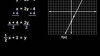
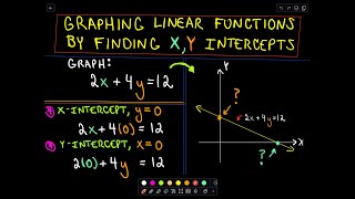
Using the x- and y- Intercepts to Graph a Linear Function
By PatrickJMT
This video shows us how to use two important features of a linear function, the x- and y- intercepts, to graph the function. Remember that we only need two points to determine a line, and often, the intercepts are extremely easy to find.
Using the x- and y- Intercepts to Graph a Linear Function
By PatrickJMT
This video shows us how to use two important features of a linear function the x- and y- intercepts to graph the function. Remember that we only need two points to determine a line and often the intercepts are extremely easy to find.


Algebra I Help: Solving Systems of Linear Equations Part II Graphing 2/3

By yourteachermathhelp
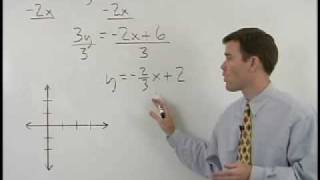
The instructor uses a white board for demonstration and this video is suitable for high school students. Students learn to solve a system of linear equations by graphing. The first step is to graph each of the given equations then find the point of intersection of the two lines which is the solution to the system of equations. If the two lines are parallel then the solution to the system is the null set. If the two given equations represent the same line then the solution to the system is the equation of that line.


Difference of Two Cubes | MathHelp.com

By MathHelp.com
To solve the given system of inequalities, we start by graphing the associated equation for each inequality. In other words, we graph y equals -1/5 x +1 and y equals 3x + 2. So, for the first inequality, we start with our y-intercept of positive 1, up 1 unit on the y-axis. From there, we take our slope of -1/5, so we go down 1 and to the right 5, and plot a second point. Now, notice that our inequality uses a “less than” sign. This means that we draw a dotted line connecting the points, rather than a solid line. It’s important to understand that if we have a greater than sign or a less than sign, we use a dotted line, and if we have a greater than or equal to sign or a less than or equal to sign, we use a solid line. Pay close attention to this idea when drawing your lines. Students often carelessly use a solid line when they should use a dotted one, and vice-versa. Next, let’s take a look at our second inequality, which has a y-intercept of positive 2, up 2 units on the y-axis. From there, we take our slope of 3, or 3 over 1, so we go up 3 and to the right 1, and plot a second point. And notice that this inequality uses a “greater than or equal to” sign, so we connect the points with a solid line, rather than a dotted line. Next, we need to determine which side of each of these lines to shade on the graph. To determine which side of our first line to shade, we use a test point on either side of the first line. The easiest test point to use is (0, 0), so we plug a zero into our first inequality for both x and y, and we have 0 is less than -1/5 times 0 + 1, which simplifies to 0 is less than 0 + 1, or 0 is less than 1. Notice that 0 is less than 1 is a true statement. This means that our test point, (0, 0), is a solution to the first inequality, so we shade in the direction of (0, 0) along our first boundary line. Next, we determine which side of our second line to shade by using a test point on either side of the second line, such as (0, 0). Plugging a zero into our second inequality for both x and y, we have 0 equal to 3 times 0 + 2, which simplifies to 0 equal to 0 + 2, or 0 equal to 2. Notice that 0 equal to 2 is a false statement. This means that our test point, (0, 0), is a not solution to the inequality, so we shade away from (0, 0) along our second boundary line. Finally, it’s important to understand that the solution to this system of inequalities is represented by the part of the graph where the two shaded regions overlap, which in this case is in the lower left. In other words, any point that lies in this part of the graph is a solution to the given system of inequalities. Note that the points along the dotted boundary line of this region are not solutions to the system, but the points along the solid boundary line of this region are solutions to the system.


ALL OF GRADE 9 MATH IN 60 MINUTES!!! (exam review part 2)

By Lumos Learning
Here is a great exam review video reviewing all of the main concepts you would have learned in the MPM1D grade 9 academic math course. The video is divided in to 3 parts. This is part 2: Linear Relations. In this video you will review everything there is to know about y=mx+b, scatterplots, and distance time graphs.

